Calibrated Uncertainty Quantification of LIFT

1 Building calibrated confidence in model predictions

For each calibration case, $x$ denotes the geometry and flow conditions, and $y$ is the corresponding reference CFD target. The target may be a field value or a derived scalar. If the model prediction is $\hat{y}(x)$, its nonconformity score is

$$s(x,y)=\frac{|y-\hat{y}(x)|}{u(x)}.$$

The term $u(x)$ sets the error scale. For deterministic inference, we set $u(x)=1$, so the score is the absolute error. This approach requires one model inference for a new geometry, making it the faster and less expensive option.

For Monte Carlo DropPath, $\hat{y}(x)$ is the mean of $T$ stochastic predictions, and $u(x)$ is their standard deviation. The score measures the prediction error relative to the sampled spread. Points with greater disagreement among the stochastic predictions receive wider intervals.

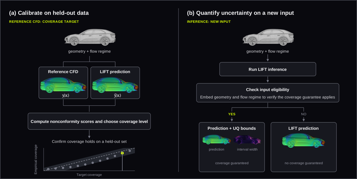
We choose a target coverage of $1-\alpha$, where $\alpha$ is the allowed error rate. For example, $\alpha =0.10$ corresponds to 90% target coverage. We compute and sort $n$ calibration scores, then set $k=\lceil (n+1)(1-\alpha )\rceil$ and take the $k$-th smallest score as $\hat{q}$. This value is the calibration threshold. A larger $\hat{q}$ means the calibration set contained larger errors relative to $u(x)$, so more margin is needed around each prediction to reach the target coverage.

For a new input $x$, the interval half-width is $\hat{q}u(x)$, giving

$$[\hat{y}(x)-\hat{q}u(x),\hat{y}(x)+\hat{q}u(x)].$$

With exchangeability and the rank choice above, this interval has finite-sample marginal coverage of at least $1-\alpha$ [2]. Exchangeability requires the calibration cases and the new input to come from the same underlying distribution of geometries and flow regimes.

The platform uses the embedding-distance check to determine whether a new input is eligible for calibration. Only an input no farther from the calibration set than the farthest sample in the coverage set receives a calibrated interval. LIFT inference still runs when this check fails, but no coverage guarantee is reported.

We calculate one calibration threshold per field rather than one per mesh point because the evaluation geometries do not share a fixed mesh. The same procedure can be applied to derived scalars, including integrated forces, moments, and aerodynamic coefficients.

2 Evaluation setup across input regimes

The Latent Interaction Field Transformer (LIFT) is UniversalAGI's in-house architecture. The rest of this article evaluates stochastic conformal intervals using a LIFT model trained on external aerodynamics simulations of cars and drones. The model predicts pressure and three wall shear stress components on the vehicle surface. Each reported prediction is the mean of ten stochastic inferences.

Calibration and coverage are evaluated on separate sets of geometries. The in-distribution (ID) set contains vehicle families represented during training. The out-of-distribution (OOD) set contains geometries and boundary conditions that differ from the training population but remain within the same physical domain of external vehicle aerodynamics. Table 1 summarizes the three calibration and evaluation experiments, including the control experiment.

Comparison	Calibration set	Evaluation set	Purpose
ID → ID	ID	ID	Baseline within a matched regime
OOD → OOD	OOD	OOD	Calibration within a new but matched regime
ID → OOD	ID	OOD	Expected failure under distribution shift

The OOD → OOD case separates the model's training distribution from the conformal calibration distribution. An input can be unfamiliar to the trained model while still belonging to the population represented by the calibration set. Coverage depends on whether the calibration set and future inputs come from the same population, not on whether that population appeared during model training.

The ID → OOD case provides a negative control. It applies calibration from one population to another, where exchangeability no longer holds and coverage is expected to fail. This comparison helps show whether the matched-regime results come from valid calibration or from intervals wide enough to cover almost any input.

We measure empirical coverage at 90% and 95% for surface pressure, the three wall shear stress components, and aerodynamic drag, CdA. Since surface points on one geometry are correlated, we use the number of geometries—not the much larger number of mesh points—to estimate the range of coverage expected from sampling variation.

3 Matched calibration preserves coverage

Figure 2 compares empirical and target coverage across the three calibration–evaluation regimes and five aerodynamic outputs.

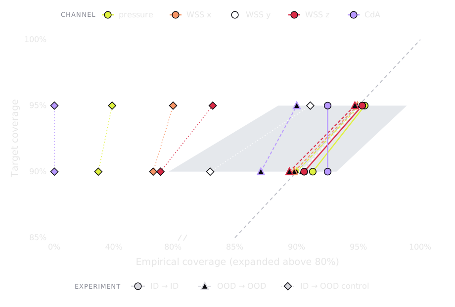
In the ID → ID evaluation, all four fields fall within the expected finite-sample range at both targets. At 90% target coverage, measured field coverage is 90.6% to 91.3%. At 95%, it is 95.3% to 95.5%. CdA coverage is 92.5% at both targets; with finite evaluation set size, that difference is consistent with sampling variation.

The OOD → OOD test gives similar results when the calibration set contains geometries and boundary conditions outside the model’s training distribution. Field coverage is 89.4% to 90.3% at the 90% target and 94.6% to 95.1% at the 95% target. CdA covers 87.1% and 90.0%, respectively. The CdA result falls just below the expected finite-sample range, but the limited evaluation-set size does not support a strong conclusion about scalar coverage.

The ID → OOD control shows the cost of using the wrong calibration data. At the 90% target, pressure coverage drops to 29.6%, and the three wall shear stress components cover 66.5% to 82.9%. The ID-calibrated CdA interval contains none of the OOD reference values. The expected failure comes from substituting calibration scores from a different geometry and flow regime.

The ID calibration fails on OOD inputs because those inputs need wider intervals. The Monte Carlo DropPath spread is too small to serve as an error bound on its own, and conformal calibration applies a larger correction for OOD inputs, especially for pressure. The spread still helps locate less certain predictions, and calibration turns that signal into useful error bounds when the calibration and input regimes match.

4 Calibrated uncertainty in practice

Calibration is performed offline for a specific model checkpoint and input regime. Held-out geometries with reference CFD simulations establish the calibration thresholds. Calibration can evolve with the application. New reference simulations can update existing thresholds or support separate calibrations for specific geometry classes and flow regimes. The platform supports deterministic bounds for lower inference cost and Monte Carlo DropPath bounds whose width varies across the surface. These options allow uncertainty estimates to be tailored to the operating regime and available computational budget.

References

1. Angelopoulos, A. N., and Bates, S. (2023). Conformal Prediction: A Gentle Introduction. Foundations and Trends in Machine Learning. https://doi.org/10.1561/2200000101.
2. Lei, J., G'Sell, M., Rinaldo, A., Tibshirani, R. J., and Wasserman, L. (2018). Distribution-Free Predictive Inference for Regression. Journal of the American Statistical Association. https://doi.org/10.1080/01621459.2017.1307116.