SUV-PT: Physics Transformer for SUVs

Highlights

• Generalization. SUV-PT generalizes across SUVs of different body types. It demonstrates impressive zero-shot generalization without fine-tuning on SUV geometries that the model has not seen.
• Fully automated large scale data collection. We created an automated, expert-validated simulation pipeline creating millions of geometries and simulations.
• Multiple global conditions.¹ SUV-PT supports a wide range of air density and inlet velocity conditions.
• Built-in uncertainty quantification. Alongside every prediction, SUV-PT outputs a per-point uncertainty quantification (see Figure 2).²
• Days → Seconds. Expert level knowledge and days of High-Performance Computing (HPC) compute for meshing + solving in traditional CFD are collapsed into seconds at a fraction of cost, and accessible to everyone.
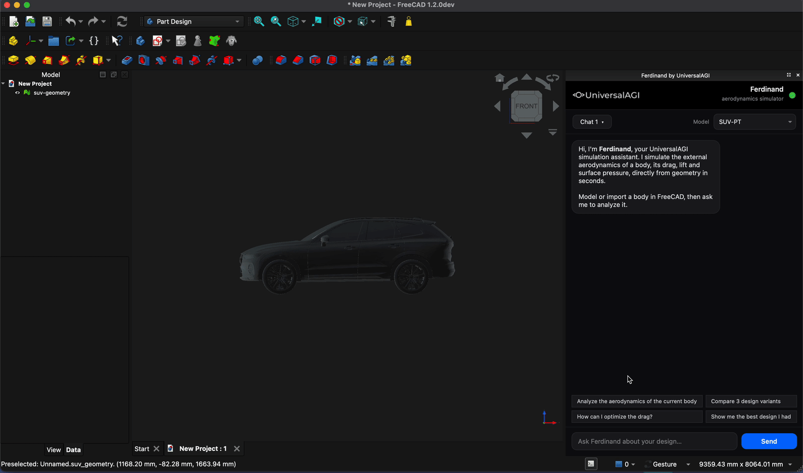
• Access. Try out SUV-PT on platform.universalagi.com, or programmatically through our API (see Appendix A4). Upload any SUV geometry and get accurate results in seconds (see Figure 1).

1 Simulation is the bottleneck in the design loop

Designing a vehicle body is an iterative loop. A designer proposes a shape. Engineers evaluate its aerodynamic performance. The result informs the next shape. The loop repeats for weeks to months, and almost all of that time goes to a single step: evaluating the design.

The most accurate way to measure a vehicle's aerodynamics is a physical wind tunnel. But that needs a built vehicle, exactly what does not yet exist during design. Modern design relies on CFD simulation instead. CFD approximates the flow around a body by solving the governing equations of fluid dynamics over a discretized model of the vehicle and the surrounding air (see Appendix A1). Accurate enough to guide design decisions without building the car, CFD has become the industry standard. Running it correctly is difficult and slow, for four main reasons.

1. Geometry cleanup. Raw CAD geometries are rarely simulation-ready. Surfaces have gaps, overlaps, and non-watertight regions that a solver cannot mesh, and removing them takes manual repair and engineering judgment before any meshing can begin.
2. Meshing. The vehicle and the space around it must be discretized into a volume of millions of cells, called a mesh. Meshing requires domain expertise, as it is error prone, and often takes several iterations of its own.
3. Configuration. A simulation cannot be set up from a fixed template. Driving it to a converged, trustworthy solution takes specialist judgment, monitoring, and revision.
4. Solve. The computation is distributed across the nodes of a high-performance computing (HPC) cluster, and even then a single high-fidelity run takes hours to days, depending on fidelity and compute.

Compute and expert time are the visible costs. In a competitive environment, the iteration cycles they impose are even more expensive. Because each evaluation takes hours to days and a trained specialist to set up, only a handful of shapes can be afforded to run simulations on. Design cycles take months, the design space is sampled sparsely, and the most efficient shape might not be among the few that are evaluated.

An ideal process would invert this. It would be accurate enough to trust, return results in seconds, and run without geometry cleanup, meshing or solver expertise. A designer could then extensively search the design space. Rather than at a few points, they can compare thousands of variants in seconds, and select the most efficient one that still meets brand identity and customer needs. Because each evaluation takes seconds, aerodynamic performance can guide the shape as it is designed, instead of being measured only after the design is finished.

2 SUV-PT predicts a vehicle's aerodynamics in seconds

As a foundational model that understands a vehicle's input geometry and its aerodynamics, SUV-PT sidesteps the need for geometry cleanup, meshing, configuration, and managed HPC. SUV-PT produces velocity fields, surface pressure, wall shear, and the integrated drag and lift in seconds. It also reports a per-point uncertainty quantification (UQ) estimate alongside each field. Figure 2 shows the surface fields for SUVs that the model has not seen. Each row compares the reference high-fidelity CFD field, SUV-PT's prediction, their difference, and SUV-PT's uncertainty quantification.

SUV-PT estimates uncertainty during inference. The resulting field is physically interpretable across the vehicle surface (see Figure 2). In the front half of the vehicle, before major separation, model uncertainty and accuracy follow the same pattern over various designs. After flow separation, the uncertainty shifts from shared-aerodynamic patterns to design-specific features, highlighting wake-sensitive components of each geometry. The uncertainty field reflects meaningful aerodynamic structure, both in attached flow regions where the flow is more constrained and in separated regions where each design produces distinct wake behavior.

2.1 SUV-PT outputs high-fidelity full field CFD

We evaluate on three benchmarks of increasing difficulty: DrivAerML [4], an open-source reference dataset; SUV-Bench Medium; and SUV-Bench Hard (see Appendix A3). We measure agreement with high-fidelity CFD using three metrics: $C_{d}A$ MAPE, the mean error on drag area (lower is better); $C_{d}A$ Max APE, the worst-case error on any single design (lower is better); and the Spearman rank correlation (higher is better), which captures whether the model ranks designs correctly (see Appendix A2).

Benchmark	CdA MAPE	CdA Max APE	Spearman Rank
DrivAerML	1.1%	3.4%	0.97
SUV-Bench Medium	2.0%	5.6%	0.96
SUV-Bench Hard	16.8%	49.1%	0.54

2.2 SUV-PT is trained in stages

We train SUV-PT in a similar way modern language models are trained. Training undergoes successive stages that move from large volumes of lower-fidelity data to volumes of high-fidelity data.

1. Lower-fidelity pre-training. The model first learns the general structure of flow over vehicle bodies from a large volume of approximate simulations.
2. High-fidelity pre-training. It is then refined on accurate, expensive simulations that resolve flow details.
3. Domain fine-tuning (optional). Finally, it can be specialized to a customer's vehicle class or operating conditions.

Across these stages, SUV-PT is trained on millions of geometries and simulations. These simulations consist of both steady-state and time series of transient-state flow fields. The model can predict both surface properties as well as volume flow distribution.³

2.3 Generating the training data is challenging

As in most of machine learning, data is a binding constraint. High-fidelity aerodynamic data does not exist publicly at the scale, diversity, and fidelity a physics model requires. So we generate it ourselves. This introduces three main challenges.

1. The data must be trustworthy. Our in-house expert simulation team produces accurate, high-fidelity, and validated data that serve as ground truth.
2. The data itself is expensive, because each run takes hours to days of compute.
3. The data is large. The full corpus spans multiple petabyte.

2.4 Training at this scale is a systems problem as much as a modeling one

A useful comparison is to modern language models. The largest corpora with trillions of tokens hardly reach the scale of petabytes. In CFD, a single training sample is a complete simulation field in space, reaching a hundred million floating point vectors, on the order of gigabytes. And because the samples are so large, the bottleneck is not only the computation. It is transferring data from storage to the GPUs fast enough to keep them utilized. The model itself adds another source of complexity. To work across, for example, vehicles, it has to handle geometries of different sizes, meshes with millions of points and different fidelities, and multiple global flow conditions.

SUV-PT is an achievement of our creative cloud infrastructure and training platform optimized for both throughput and resilience, churning through petabytes of data across multiple GPU nodes.

3 LIFT is faster and more accurate than existing state-of-the-art physics models

To place our LIFT architecture in context, we compared it against the existing state-of-the-art physics models GeoTransolver [1] and Transolver [2]. Every model was given the same number of parameters, so the comparison reflects the architecture rather than its scale. A training epoch is one pass over each sample at a downsampled input resolution, while inference is run on the full sample.

On a single Nvidia A100 GPU, LIFT is the fastest to train and to serve, the former measured on a reduced training set, and it has the smallest memory footprint (see Table 2). Because GPU memory is a binding constraint, we also report training throughput per unit of peak memory, where LIFT is 5x more efficient than state-of-the-art architectures.

Architecture	P50 Inference latency	Training throughput	Peak GPU memory	Throughput / memory
LIFT	10.2 s	0.93 (samples/s)	13.9 GiB	0.067 samples/s/GiB
Transolver [2]	19.7 s	0.45 (samples/s)	21.1 GiB	0.021 samples/s/GiB
GeoTransolver [1]	23.6 s	0.41 (samples/s)	23.0 GiB	0.018 samples/s/GiB

3.1 Training time: LIFT reaches the same loss in less wall-clock time

Holding the model size fixed, we trained each architecture on a reduced set to the same loss target and recorded wall-clock time. At a batch size of one, LIFT achieves 2.3x and 2.1x the throughput of GeoTransolver [1] and Transolver [2], respectively (see Figure 3).

3.2 Inference latency: LIFT outperforms the state-of-the-art

We measured single-sample inference latency on DrivAerML [4] surface data, using one NVIDIA A100 GPU per model and timing the forward pass only (see Figure 4). We report the latency distribution with its median (P50) and tails (P90, P95). LIFT has the lowest latency at every percentile, with a median of 10.2 s against 19.7 s for Transolver [2] and 23.6 s for GeoTransolver [1].

4 SUV design in seconds

SUV-PT is served through a project-based platform and API. Each project holds a set of geometries and the conditions they are evaluated under. Within a project, a user can run a parameter sweep¹ across multiple boundary conditions and geometries and obtain results in seconds. The platform supports the comparisons a CAD workflow relies on. For example, variants placed side by side and profile distributions along the body. Results can be exported for downstream use. The same workflow is available through our API, so a geometry optimization procedure can infer SUV-PT directly and evaluate thousands of variants in seconds (see Appendix A4).

5 Availability

SUV-PT is live on our platform. Upload an SUV geometry and get its aerodynamics in under a minute. Open the platform to evaluate your own designs, and contact us to discuss deployments or domain customization for your use case.

---

1. The current public preview exposes a single condition set. The entire condition set is included with full model access.
2. UQ is included with full model access.
3. This release exposes the surface fields. Surface and volume fields are included with full model access.

Appendix

A1 CFD and meshing

CFD is used across many engineering and biomedical domains, including aircraft design, turbomachinery, building ventilation, and cardiovascular flow modeling. Here, we focus on vehicle aerodynamics, where CFD provides a numerical alternative to wind-tunnel testing. Rather than measuring airflow around a physical prototype, CFD solves discretized governing equations over a computational mesh to approximate the velocity and pressure fields around the vehicle.

At typical road speeds, vehicle aerodynamics is well described by the incompressible-flow approximation. Under this assumption, the fluid motion is governed by the incompressible Navier-Stokes equations:

$$\nabla ·\mathbf{u}=0,$$ $$\rho (\frac{\partial \mathbf{u}}{\partial t}+(\mathbf{u}·\nabla )\mathbf{u})=-\nabla p+\mu {\nabla }^2\mathbf{u}+\mathbf{f}.$$

Here $\mathbf{u}$ denotes the velocity field, $p$ the pressure, $\rho$ the fluid density, $\mu$ the dynamic viscosity, and $\mathbf{f}$ an external body-force field. The first equation enforces mass conservation. For an incompressible fluid, air neither accumulates nor vanishes within the domain. The second equation enforces momentum conservation, balancing acceleration with pressure gradients, viscous stresses, and external body forces. Once the solver approximates the pressure and shear-stress distributions on the vehicle surface, drag can be computed by integrating those surface forces.

The governing equations are continuous, but a computer can only solve a finite-dimensional approximation. A CFD solver discretizes the air volume surrounding the vehicle into a mesh and computes the flow variables. Mesh design is one of the central engineering decisions in high-fidelity CFD. Cells must be fine enough near the vehicle surface, across the boundary layer, around wheel wakes, and in separated-flow regions behind the vehicle. If critical regions are under-resolved, the solver may converge to a numerically precise but physically inaccurate solution. If the mesh is refined everywhere, the simulation becomes unnecessarily expensive. Equally important is mesh quality, as poorly shaped or highly skewed cells can degrade numerical accuracy and compromise solver stability.

Even with a well-designed mesh, directly resolving the Navier-Stokes equations across all relevant turbulent scales is usually too expensive for full-vehicle aerodynamics. The smallest turbulent structures can be orders of magnitude smaller than the vehicle-scale flow features, so resolving them everywhere would require a prohibitive number of cells and time steps. Turbulence models address this gap by modeling part of the turbulent motion rather than resolving every scale directly. This choice strongly affects the mesh and compute budget. Reynolds-averaged Navier-Stokes models reduce cost by modeling most turbulent fluctuations and can often use coarser meshes, especially away from walls. Large eddy simulation and detached eddy simulation resolve more unsteady turbulent structures, but they require finer grids, smaller time steps, and greater computational cost. Every modeling choice therefore balances accuracy, cost, and the physics captured.

A2 Evaluation metrics

We report three metrics on drag area, $C_{d}A$. Let $y_i$ be the CFD value for design $i$, ${\widehat{y}}_i$ be the model prediction, and $N$ be the number of designs.

Mean absolute percentage error (lower is better) measures average relative error:

$$\text{MAPE}=\frac{100}{N}\sum _{i=1}^N\left|\frac{y_i-{\widehat{y}}_i}{y_i}\right|.$$

Max absolute percentage error (lower is better) measures the worst prediction:

$$\text{max APE}=100·\underset{i}{max}\left|\frac{y_i-{\widehat{y}}_i}{y_i}\right|.$$

Spearman rank correlation (higher is better) measures whether the model orders designs accurately:

$$\rho =1-\frac{6\sum _{i=1}^N{d}_i^2}{N(N^2-1)},d_i=\text{rank}\left({\widehat{y}}_i\right)-\text{rank}\left(y_i\right).$$

A3 Benchmarks

We use three benchmarks:

• DrivAerML [4] is a public and well known, high-fidelity CFD dataset built around the DrivAer reference body.
• SUV-Bench medium contains production-like SUV geometries with moderate variation.
• SUV-Bench hard contains production-like SUV geometry outliers with unrealistically mutated geometry features (see Figure 5).

A4 API and CAD software access for geometry optimization

The API is useful when an evaluation becomes a search over thousands of geometries and operating conditions. A geometry optimization procedure can generate a batch of variants, infer SUV-PT on each one, and rank the candidates by drag without manual geometry cleanup, meshing, solver setup, or managing the HPC. The operating conditions can be swept, for example multiple inlet velocities, or fixed with a single value.

from universalagi import UniversalAGI, DesignScores, GeometrySet, OperatingConditions, Range, Value

client = UniversalAGI()  # reads UAGI_API_KEY from the environment

geometries = GeometrySet.from_paths([
    "variants/suv_001.stl",
    "variants/suv_002.stl",
    "variants/suv_003.stl",
    "...",
    "variants/suv_n.stl",
])

conditions = OperatingConditions(
    velocity=Range(25.0, 40.0, steps=1000),
    air_density=Value(1.225),
)

simulation = client.simulate(
    model="suv-pt-1",
    geometries=geometries,
    conditions=conditions,
)

scores = DesignScores.from_simulation(simulation, metric="CdA")
best_geometry = scores.best()
print(best_geometry.path, best_geometry.value)

Each prediction returns integrated aerodynamic quantities such as $C_{d}A$, $C_D$, and $C_L$. The full surface and volume fields can also be exported to standard mesh formats (e.g., vtu, vtp, stl, cgns) for inspection in tools such as ParaView. The same API can be called from extensions or automation scripts inside CAD environments such as CATIA, Autodesk, FreeCAD, or SolidWorks. This enables designers to make aerodynamically informed decisions without leaving their workflow (see Figure 6).

References

1. Adams, C., Ranade, R., Cherukuri, R., & Choudhry, S. (2025). GeoTransolver: Learning Physics on Irregular Domains Using Multi-scale Geometry Aware Physics Attention Transformer. arXiv preprint arXiv:2512.20399.
2. Wu, H., Luo, H., Wang, H., Wang, J., & Long, M. (2024). Transolver: A fast transformer solver for pdes on general geometries. arXiv preprint arXiv:2402.02366.
3. Xue, L., Yu, N., Zhang, S., Panagopoulou, A., Li, J., Martín-Martín, R., ... & Savarese, S. (2024). Ulip-2: Towards scalable multimodal pre-training for 3d understanding. In Proceedings of the IEEE/CVF Conference on Computer Vision and Pattern Recognition (pp. 27091-27101).
4. Ashton, N., Mockett, C., Fuchs, M., Fliessbach, L., Hetmann, H., Knacke, T., ... & Maddix, D. (2024). DrivAerML: High-fidelity computational fluid dynamics dataset for road-car external aerodynamics. arXiv preprint arXiv:2408.11969.