Epistemic Uncertainty in LIFT with Monte Carlo Sampling

1 Sampling different paths through one model

A direct way to estimate epistemic uncertainty is to train several models independently and compare their predictions. Deep ensembles capture differences caused by random initialization and training [2], but each model requires a separate training run, checkpoint, and inference pass.

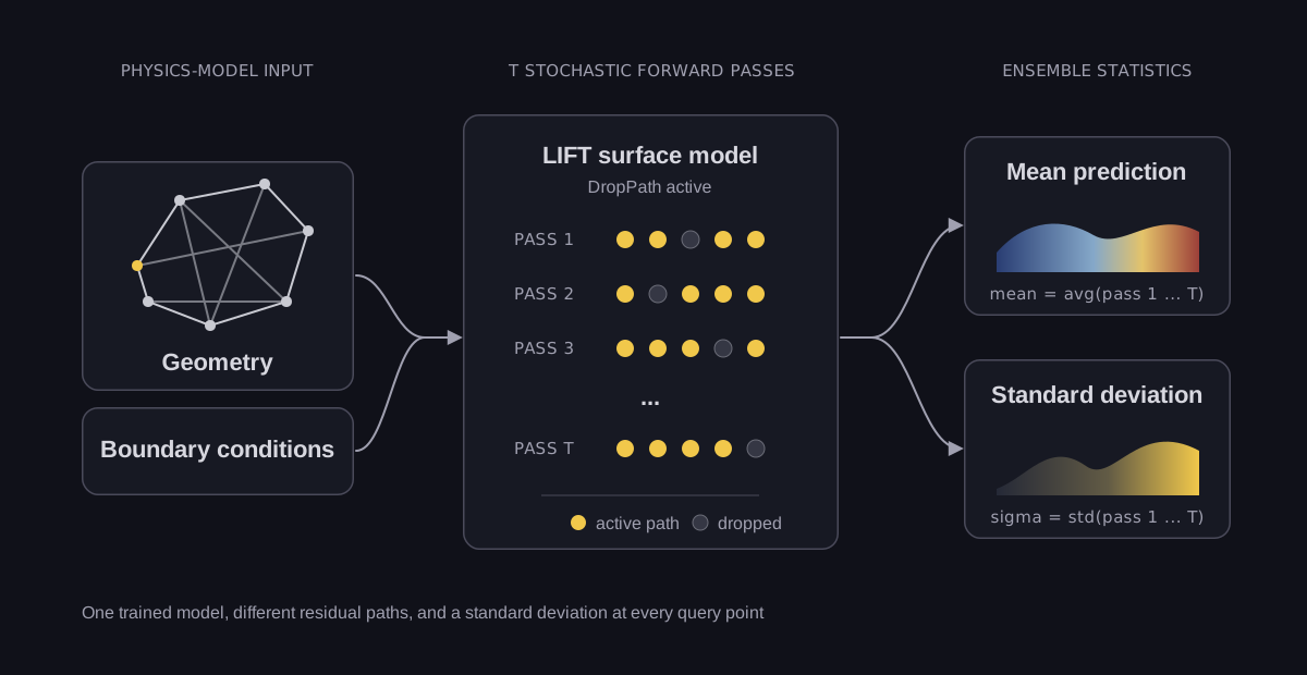
Monte Carlo dropout samples different activation masks across repeated passes through one trained network [3]. We apply the same approach to LIFT's DropPath layers. Each pass samples complete residual branches instead of individual activations [4]. Averaging the stochastic passes gives the Monte Carlo mean prediction. Their spread shows how strongly that prediction depends on the sampled path and serves as a proxy for epistemic uncertainty. Such stochastic sampling should not increase prediction error. We compare the Monte Carlo mean with standard deterministic inference before interpreting the spread.

Let $y_t$ be the field from stochastic pass $t$. For $T$ passes, the Monte Carlo mean is

$$\overline{y}=\frac{1}{T}\sum _{t=1}^T{y}_t,$$

and the path-wise standard deviation is

$${\sigma }_{\text{epistemic}}={\left[\frac{1}{T-1}\sum _{t=1}^T{(y_t-\overline{y})}^2\right]}^{\frac{1}{2}}.$$

Each LIFT inference returns one physical field. After $T$ stochastic inferences, we compute the mean and path-wise standard deviation at every query point as a post-processing step. This is an ensemble over paths, not independently trained models. All passes share the same learned weights and training data. Monte Carlo DropPath is cheaper to train and store than a deep ensemble. A deep ensemble can disagree because each member learned different weights. DropPath can disagree only because different residual branches were dropped.

2 SUV-PT: A benchmark of Monte Carlo DropPath

SUV-PT is one physics model built on LIFT. Its surface model predicts pressure and wall shear stress from vehicle geometry and operating conditions. Repeated stochastic passes produce a mean prediction and a standard deviation value at every point on the vehicle surface for each predicted field.

We judge the method on three practical tests:

• The Monte Carlo mean must preserve deterministic accuracy.
• The path-wise standard deviation should rise on unfamiliar inputs.
• The path-wise standard deviation should be greater where field error is larger.

We group the evaluation sets as in-distribution (ID), out-of-distribution (OOD), and out of domain. ID inputs come from the same population as the training data. OOD inputs remain in the automotive domain but differ from the training population. Out-of-domain inputs come from a different physics domain.

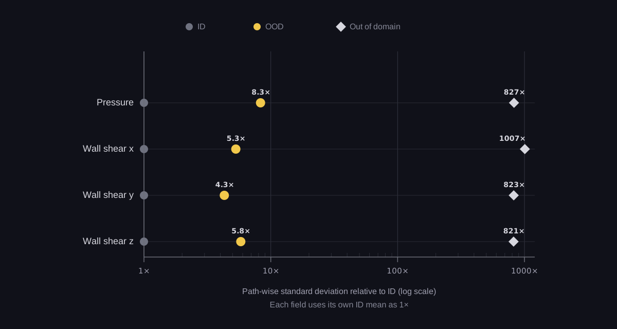
On the ID evaluation, field errors changed by less than 0.3%, while error in the integrated quantity of interest decreased by 2.2% relative to deterministic inference. The additional sampling added an uncertainty signal without degrading the point prediction. Relative to ID, mean path-wise standard deviation across the four predicted fields was 4.3 to 8.3 times higher on OOD inputs and 821 to 1,007 times higher on out-of-domain inputs. Figure 2 plots that comparison on a logarithmic axis. In practice, a large spread tells engineers when to check a prediction with CFD.

The spread is not a single number for the vehicle. It varies over the surface. Figure 3 shows two SUV-PT examples. Each row compares a reference CFD simulation, the LIFT model prediction, the absolute error, and the Monte Carlo DropPath standard deviation.

Across the surface evaluation, path-wise standard deviation and absolute error had a positive Pearson correlation for every predicted field: cells with greater path disagreement tended to have higher error. The spread broadly tracked where errors occurred, but its raw magnitude was smaller. The spread is a relative signal, not a calibrated error bar.

3 Where to allocate the CFD budget

The spread gives the engineer a way to rank predictions for further review. Agreement between sampled paths supports using the physics-model prediction. Strong disagreement points to cases, or regions of a surface, where another CFD simulation can be informative. A geometry parameter is a scalar that controls one named feature of the vehicle shape, such as side mirror height. The rest of the vehicle stays fixed. Figure 4 illustrates a sweep of one such parameter. Each design variant receives ten stochastic CdA predictions, and variants with the widest spread receive higher CFD priority.

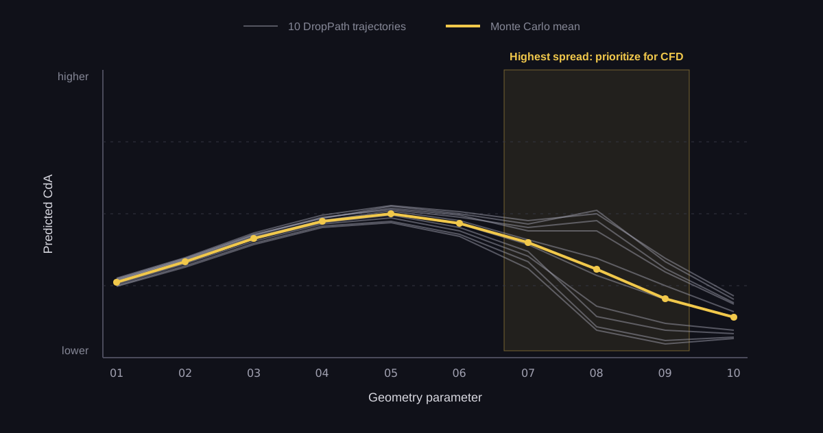
Monte Carlo DropPath adds an uncertainty field to every physics-model prediction without a second training run. Engineers can keep the model prediction when sampled paths agree, and send the high-spread cases to a CFD solver. The same simulation budget then covers more of the design space.

References

1. Kendall, A., and Gal, Y. (2017). What Uncertainties Do We Need in Bayesian Deep Learning for Computer Vision? Advances in Neural Information Processing Systems. https://arxiv.org/abs/1703.04977.
2. Lakshminarayanan, B., Pritzel, A., and Blundell, C. (2017). Simple and Scalable Predictive Uncertainty Estimation using Deep Ensembles. Advances in Neural Information Processing Systems. https://arxiv.org/abs/1612.01474.
3. Gal, Y., and Ghahramani, Z. (2016). Dropout as a Bayesian Approximation: Representing Model Uncertainty in Deep Learning. International Conference on Machine Learning. https://arxiv.org/abs/1506.02142.
4. Huang, G., Sun, Y., Liu, Z., Sedra, D., and Weinberger, K. Q. (2016). Deep Networks with Stochastic Depth. European Conference on Computer Vision. https://doi.org/10.1007/978-3-319-46493-0_39.